With the kind of data that I usually work with, overfitting regression models can be a huge problem if I’m not careful. Ridge regression is a really effective technique for thwarting overfitting. It does this by penalizing the L2 norm (euclidean distance) of the coefficient vector which results in “shrinking” the beta coefficients. The aggressiveness of the penalty is controlled by a parameter
Lasso regression is a related regularization method. Instead of using the L2 norm, though, it penalizes the L1 norm (manhattan distance) of the coefficient vector.
Because it uses the L1 norm, some of the coefficients will shrink to zero while lambda increases. A similar effect would be achieved in Bayesian linear regression using a Laplacian prior (strongly peaked at zero) on each of the beta coefficients. Because some of the coefficients shrink to zero, the lasso doubles as a crackerjack feature selection technique in addition to a solid shrinkage method. This property gives it a leg up on ridge regression. On the other hand, the lasso will occasionally achieve poor results when there’s a high degree of collinearity in the features and ridge regression will perform better. Further, the L1 norm is underdetermined when the number of predictors exceeds the number of observations while ridge regression can handle this.
Elastic net regression is a hybrid approach that blends both penalization of the L2 and L1 norms. Specifically, elastic net regression minimizes the following…
the
The usual approach to optimizing the lambda hyper-parameter is through cross-validation—by minimizing the cross-validated mean squared prediction error—but in elastic net regression, the optimal lambda hyper-parameter also depends upon and is heavily dependent on the alpha hyper-parameter (hyper-hyper-parameter?).
This blog post takes a cross-validated approach that uses grid search to find the optimal alpha hyper-parameter while also optimizing the lambda hyper-parameter for three different data sets. I also compare the performances against the stepwise regression and showcase some of the dangers of using stepwise feature selection.
mtcars
In this example, I try to predict “miles per gallon” from the other available attributes. The design matrix has 32 observations and 10 predictors and there is a high degree of collinearity (as measured by the variance inflation factors).
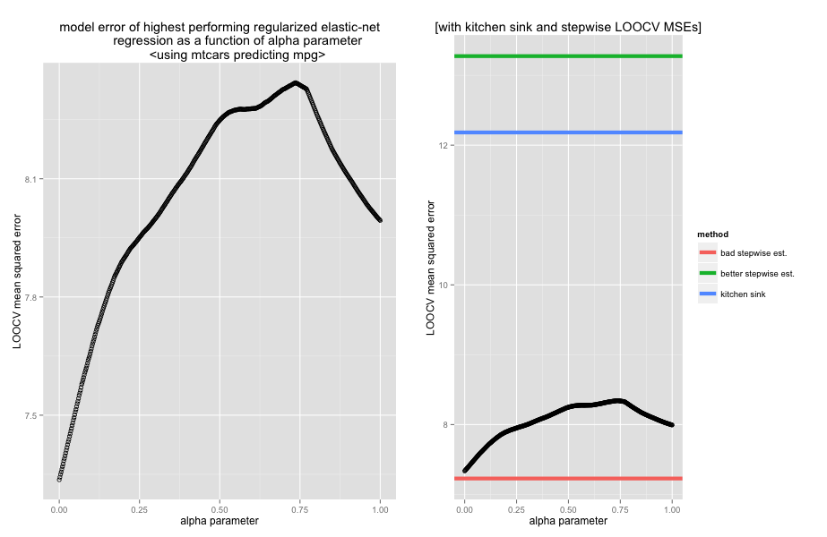 The left panel above shows the leave-one-out cross validation (LOOCV) mean squared error of the model with the optimal lambda (as determined again by LOOCV) for each alpha parameter from 0 to 1. This panel indicates that if our objective is to purely minimize MSE (with no regard for model complexity) than pure ridge regression outperforms any blended elastic-net model. This is probably because of the substantial collinearity. Interestingly, the lasso outperforms blended elastic net models that weight the lasso heavily.
The right panel puts things in perspective by plotting the LOOCV MSEs along with the MSE of the “kitchen sink” regression (the blue line) that includes all features in the model. As you can see, any degree of regularization offers a substantial improvement in model generalizability.
It is also plotted with two estimates of the MSE for models that blindly use the coefficients from automated bi-directional stepwise regression. The first uses the features selected by performing the stepwise procedure on the whole dataset and then assesses the model performance (the red line). The second estimate uses the step procedure and resulting features on only the training set for each fold of the cross validations. This is the estimate without the subtle but treacherous “knowledge leaking” eloquently described in this plot post. This should be considered the more correct assessment of the model. As you can see, if we weren’t careful about interpreting the stepwise regression, we would have gotten an incredibly inflated and inaccurate view of the model performance.
Forest Fires
The second example uses a very-difficult-to-model dataset from University of California, Irvine machine learning repository. The task is to predict the burnt area from a forest fire given 11 predictors. It has 517 observations. Further, there is a relatively low degree of collinearity between predictors.
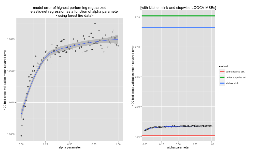
Again, highest performing model is the pure ridge regression. This time, the performance asymptotes as the alpha hyper-parameter increases. The variability in the MSE estimates is due to the fact that I didn’t use LOOCV and used 400-k CV instead because I’m impatient.
As with the last example, the properly measured stepwise regression performance isn’t so great, and the kitchen sink model outperforms it. However, in contrast to the previous example, there was a lot less variability in the selected features across folds—this is probably because of the significantly larger number of observations.
“QuickStartExample”
This dataset is a contrived one that is included with the excellent glmnet package (the one I’m using for the elastic net regression). This dataset has a relatively low degree of collinearity, has 20 features and 100 observations. I have no idea how the package authors created this dataset.
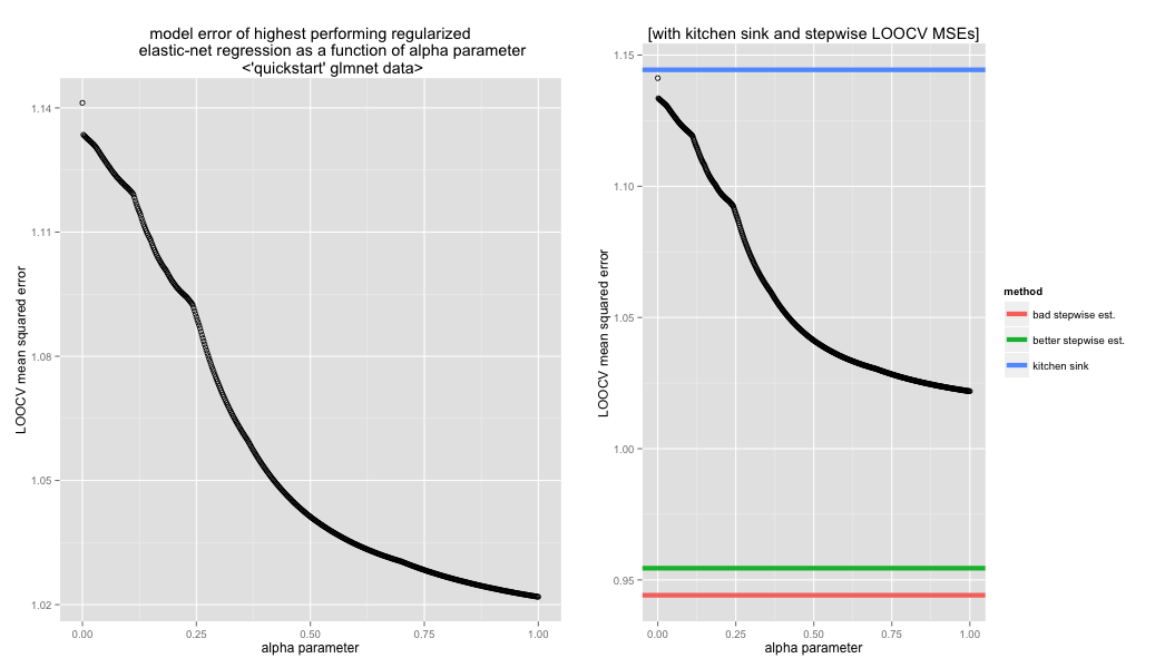
Finally, an example where the lasso outperforms ridge regression! I think this is because the dataset was specifically manufactured to have a small number of genuine predictors with large effects (as opposed to many weak predictors).
Interestingly, stepwise progression far outperforms both—probably for the very same reason. From fold to fold, there was virtually no variation in the features that the stepwise method automatically chose.
Conclusion
So, there you have it. Elastic net regression is awesome because it can perform at worst as good as the lasso or ridge and—though it didn’t on these examples—can sometimes substantially outperform both.
Also, be careful with step-wise feature selection!
PS: If, for some reason, you are interested in the R code I used to run these simulations, you can find it on this GitHub Gist.